Realizing string-net condensation: Fibonacci anyon braiding for universal gates and sampling chromatic polynomials

The DSNP strategy

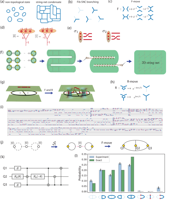
Our approach to creating minimalistic Fib-SNC is the scalable dynamic string-net preparation (DSNP) strategy (see Fig. 1f). As explained below, we implement this strategy to create τ1 anyons, confirm their anyon charges, and braid them to extract the golden ratio. Furthermore, DSNP allows us to make the first steps towards scaling up the Fib-SNC to estimate the chromatic polynomial at the golden ratio ϕ + 2.

DSNP leverages the inherent flexibility of graphs for efficient dynamical preparation of the Fib-SNC (see Fig. 1f). This is in contrast to the proposal of operating on a rigid lattice^26,27. A similar graph-centric perspective has proven productive for preparing states with Ising anyons²⁸. A single physical qubit can represent the smallest isolated string-net, or ‘bead’, when prepared in a valid superposition through the modular-\({\mathcal{S}}\) gate:

The next step in building a larger-scale Fib-SNC is to insert a qubit initialized in the \(\left\vert 0\right\rangle\) state between beads. Using F-moves (see Fig. 1c), the beads can be entangled into a strip of plaquettes. This strip can then be folded and sewn into a two-dimensional Fib-SNC through additional F-moves. The dynamic nature of this process allows for the optimization of resources for specific aims. The depth of the circuit grows linearly with the system size, the best scaling expected for a unitary circuit preparation of a topologically ordered state²⁹, but with the smallest prefactor to our knowledge compared to previous proposals, such as ref. ²⁷. To prepare the Fib-SNC with N × N plaquettes, ref. ²⁷ estimated  ≈ 120N layers of parallel CNOTS. With DSNP, the required depth scales as 2N 5-qubit F-moves. Using a conservative estimation of 40 CNOTs per 5-qubit F-moves²⁷, the depth of the DSNP scales as 80N CNOT layers, with all other steps being parallelizable.

Creation of anyons must change the topology of the many-body state. In order to establish a protocol that allows explicit association between the circuit implementation and the evolving topology of the many-body state, we introduce a three-dimensional (3D) graphical representation where each copy of the TQFT is depicted as a two-dimensional surface (see Fig. 1g). While the anyon-free Fib-SNC can be visualized entirely through two-dimensional (2D) graphs, the creation of anyons whose ‘anyon charge’ labels which of the two copies of TQFT is affected necessitates keeping track of the two copies. Anyons connect the two surfaces through ‘worm holes’ at the locations of anyons. Furthermore, to create anyons while allowing for the detection and correction of local errors, we follow the ‘tail anyon’ strategy²⁰ that traps the end of an open string to the ‘tail qubit’ located on a dangling edge inside a plaquette. The τ1 or 1τ pair-creation can now be visualized as bringing in an open string from above or below the two surfaces. Fig. 1g illustrates inserting the strings from above into the Fib-SNC state shared between the two surfaces, which requires undoing the over-crossing using the ‘R-move’ shown in Fig. 1h.

As a flexible state preparation strategy built on graphs, DSNP allows the preparation of Fib-SNC with an arbitrary number of plaquettes. The smallest of such only requires three qubits forming two plaquettes, which can be prepared as shown in Fig. 1j using a circuit with two \({\mathcal{S}}\) gates and a three-qubit F-move shown in Fig. 1k (see “Methods” for more details). Fig. 1l shows the experimental result of implementing this Fib-SNC on the 27-qubit IBM Falcon processor ibm_peekskill. Using dynamical decoupling and readout-error mitigation³⁰, but without other error mitigation, we sample the probability distribution of computational bitstrings using 8192 experimental shots. The x-axis labels represent bitstrings as their corresponding graph configurations, with dashed (solid) lines indicating qubits in the \(\left\vert 0\right\rangle\) (\(\left\vert 1\right\rangle\)) state and red  × ’s denoting broken strings. Full tomography reconstruction of the experimental state yields a fidelity of 0.87 ± 0.01 to the ideal state, which is not high in the absolute sense. However, the state shows a much higher degree of 95% adherence to the branching rule.

Anyon creation and certification

Now we create a pair of Fibonacci anyons and certify their anyon types in the above two-plaquette Fib-SNC state. To create the τ1 pair, we introduce an open string (red) of qubits (Q5 and Q7) above the two-plaquette Fib-SNC (Fig. 2a). With an unoccupied string (Q6 initialized in state \(\left\vert 0\right\rangle\)) as the bridge, we entangle the open string with the Fib-SNC via F-moves and an R-move as illustrated in Fig. 2a–c (see “Method” for details). These moves restore the planarity of the graph and effectively create two wormholes connected by an open string through the upper-copy TQFT. Now, both plaquettes each host a τ1 anyon at the tail. Although the qubits, except the tail qubits, now respect the local rules of Fib-SNC, the two copies of the TQFT share a complex superposition through the wormholes. To create the other anyon type, the 1τ anyons, the open string should be inserted from underneath the two-plaquette Fib-SNC rather than from above. Practically, this amounts to using the conjugate R^*-move instead of the R-move.

a–c Building a minimal two-plaquette string-net and creating a pair of τ1 anyons. a Qubits Q1–Q4 are initialized in \(\left\vert 0\right\rangle\) encoding an empty two-plaquette graph, Q5 and Q7 initialized in \(\left\vert 1\right\rangle\) support the open string in the upper sheet. Q6 in \(\left\vert 0\right\rangle\) is an ancillary unoccupied string segment. b An F-move transforms the graph into a 3D configuration. c An R-move on Q6 yields a pair of τ1 anyons localized on the left and right plaquettes, with Q5 and Q7 acting as their tail qubits. The resulting open string threads through the upper plane, with its two ends supporting the τ1 anyons that pierce the two wormholes in the sheets (recall Fig. 1g). One further applies F-moves flipping edge Q2 and Q4 to reach the configuration in (d). d, e The anyon type is diagnosed by a charge measurement performed using a further F-move flipping edge Q6 to deform the graph into two connected plaquettes (e), joined at Q6. f Unitaries U act on pairs (Q4, Q1) and (Q2, Q3) to place Q4 and Q2 on the open string. g The circuit for the anyon type certification. h The compilation of the unitary U with three 2-qubit ECR gates (See SM Sec. VI) and a few single-qubit gates for the 2-qubit unitary U. i The contrast experiment prepares a pair of 1τ anyons by replacing the R-move with its complex conjugate. Thus, in the final measurement stage, the open string goes through the bottom plane with qubits Q1 and Q3 in its path. j Theory (gray bars) vs. experiment (colored bars) for the τ1 (left) and 1τ (right) anyon pairs measured in the 2D graph in panel (e) before applying U(upper) and the 3D graph in panel (f) after applying U(lower). The expectation values \(\left\langle \,| 1\right\rangle \left\langle 1| \,\right\rangle\) are indistinguishable in the 2D graph. However, in the 3D graph, the \(\left\vert 1\right\rangle\)-state expectation values of unpinned qubits Q1–4 certify the anyon type as the measurement reveals the path of the open string.

The canonical way to certify the anyon type would be to measure the five-qubit plaquette operators for each plaquette in the two-dimensional graph in Fig. 2c. However, to combat the noise obscuring the certification in such extended measurements, we introduce an alternative approach that reduces this certification to independent single-qubit measurements. We first deform the graph so that the open string is pinned in the middle to be shared between the two TQFT’s, as shown in Fig. 2e. Now, each plaquette can be independently measured, while the two tail qubits (Q5 and Q7) and the qubit bridging the plaquettes (Q6) are fixed to be in the \(\left\vert 1\right\rangle\) state, irrespective of the anyon type τ1 or 1τ. At this point, all the qubits are still shared between the two TQFT’s and we referred to this state as “2D graph”. We then lift the remaining four qubits off the shared space through a basis-changing unitary represented as U. In the end, the open string passes through all but two of the qubits. In particular, measurements of lifted qubits (Q1, Q4, Q2, Q3) in the final “3D graph” shown in Fig. 2f for τ1’s amount to measuring the open string itself with a definite parity associated with the anyon types (see “Method” for details on the implementation of Fig. 2e, f).

To experimentally realize the anyon pair preparation and the anyon charge measurements, we need high-accuracy circuits about 150 two-qubit-gate-layers deep. We use a 133-qubit IBM Heron processor ibm_torino, featuring fast gates and reduced cross-talk, with median single- and two-qubit gate fidelities of 3.6 × 10⁻⁴ and 4.6 × 10⁻³, respectively (see SM Sec. VI). To address experimental noise, we employ a composite error suppression and mitigation strategy, including real-time qubit selection, dynamical decoupling, twirling^31,32, zero-noise extrapolation^33,34,35, and twirled readout-error mitigation³⁰ (see SM Sec. VII).

We now create pairs of each anyon type and certify their type through single qubit measurements over 8.8 × 10⁶ experimental realizations across 1100 quantum circuit instances (see SM Sec. VIII). In Fig. 2j shows the resulting measurement outcome statistics for each of the qubits corresponding to the two anyon types. We measured 2D graphs like Fig. 2e and 3D graphs like Fig. 2f. The measurement results shown in Fig. 2j confirm the prediction with high precision. Specifically, three pinned qubits Q5–7 are consistently measured in the \(\left\vert 1\right\rangle\) state at all times. In the 2D graph, although single-qubit measurements hide the anyon type even for the remaining four qubits (Q1–4), the measured expectation value of \(\left\langle \,| 1\right\rangle \left\langle 1| \,\right\rangle\) of 0.73 ± 0.04 as shown in the upper histograms in Fig. 2j is consistent with the theoretically predicted value of \(\frac{{\phi }^{2}}{{\phi }^{2}+1}\approx 0.72\). However, these four qubits (Q1–4) show a dramatic contrast between the two anyon types in 3D graphs, as shown in the lower histograms in Fig. 2j. Since these four qubits are “lifted off” the shared plane to belong to top or bottom TQFT, the open string traverses the top TQFT with Q4 and Q2 (τ1) or the bottom TQFT with Q1 and Q3 (1τ) depending on the anyon type. (see Method for more details).

Braiding doubled Fibonacci anyons

Fully two-dimensional braiding must involve three or more plaquettes and two pairs of τ1 anyons. DSNP prescribes a scalable strategy for creating plaquette strips of arbitrary lengths. In Fig. 3, we demonstrate two-dimensional braiding in a scalable and error-correctable manner using the minimalistic three-plaquette strip and verify the braiding outcome through the fusion of a pair of anyons (see Fig. 3a for the schematics). Repeating the anyon pair preparation, we prepare two anyon pairs spread over three plaquettes as depicted in Fig. 3b. This amounts to time steps t₀–t₁ in Fig. 3a. Initially, the logical qubit encoded to the triplet of τ1 anyons (1,2,3) is in the \(\overline{\left\vert 0\right\rangle }\) state since the anyon 1 and anyon 2 are created from vacuum. Now, we braid τ1 anyons 2 and 3 using a sequence of exact F-moves executing the time steps t₁–t₂ in Fig. 3a. Such braiding is predicted to execute a non-Clifford gate σ₂ (see Fig. 1e) on the logical qubit, rotating the logical state to

We certify the predicted non-Clifford gate by fusing anyon 1 and anyon 3. For this, we bring anyon 1 and anyon 3 together to share a single root edge using an R-move and an F-move(see Fig. 3e). Now a measurement in the physical computational basis of the root edge onto either \(\left\vert 0\right\rangle\) or \(\left\vert 1\right\rangle\) projects the logical qubit to \(\overline{\left\vert 0\right\rangle }\) or \(\overline{\left\vert 1\right\rangle }\), respectively. Hence, if the braiding implements the correct logical gate in Eq. (2), the golden ratio can be measured through \(\left\langle \,| 1\right\rangle \left\langle 1| \,\right\rangle /\left\langle \,| 0\right\rangle \left\langle 0| \,\right\rangle=\phi\).

As in the previous experiment, we implement this sequence on ibm_torino using the composite mitigation strategy, but with double the number of twirls and shots per twirl due to the increased circuit complexity. We find \(\left\langle \,| 1\right\rangle \left\langle 1| \,\right\rangle /\left\langle \,| 0\right\rangle \left\langle 0| \,\right\rangle=1.65\pm 0.14\), within 2% of the golden ratio ϕ. Figure 3g shows the distribution of bootstrap resampling, providing confidence intervals (see SM Sec. VIII). In a control experiment, we intentionally introduce bit-flip errors during to break two strings, generating unwanted excitations (see SM Sec. VIII). This modification alters the bitstring distribution. We now measure \(\left\langle \,| 1\right\rangle \left\langle 1| \,\right\rangle /\left\langle \,| 0\right\rangle \left\langle 0| \,\right\rangle=0.30\pm 0.025\), consistent with the theoretical prediction of 0.328 for the modified circuit.

a Worldlines depicting the creation of four τ1 anyons from the vacuum 11, followed by the braiding of anyons 2 and 3, and concluding with a fusion-based measurement to determine the logical gate implemented by the braiding process. b Generalization of the protocol from Fig. 2, where four τ1 anyons (red dots labeled as 1–4) are initialized on three plaquettes. Labels for the qubits (yellow dots) are suppressed. c, d Braiding is achieved through four five-qubit F-moves, which permute anyons 2 and 3. The groups of five qubits undergoing the F-moves are indicated by the orange patches. e An R-move flips anyon 3 from the center to the left plaquette, forming a new configuration for fusion. f A final F-move fuses anyons 1 and 3, resulting in a coherent superposition of two fusion outcomes. g Experimental distributions of the measured ratio \(\left\langle 1| 1\right\rangle /\left\langle 0| 0\right\rangle\) on a logarithmic scale, derived via bootstrap resampling for both the braiding and control experiments. The analysis accounts for error mitigation and statistical uncertainty (see SM Sec. VIII). Vertical dashed lines indicate theoretical predictions: the golden ratio ϕ (yellow) and the control value (purple). Asymmetry in the distributions reflects the non-linear transformation of the ratio observable.

Estimating the chromatic polynomials via string-net sampling

Now we move onto the most ambitious pursuit of this paper, taking the first step towards a new class of classically hard problems. In Fig. 4, we realize a two-dimensional, four-plaquette Fib-SNC vacuum and sample it to estimate the chromatic polynomials for all possible trivalent graph embedding. We perform all experiments on ibm_torino. Due to the outstanding challenge of mitigating noise for sampling rather than expectation values³⁵, we only mitigate readout errors and not gate errors. We use DSNP as illustrated in Fig. 4a–d, starting with a four-bead strand and evolving each bead into one of the four-plaquettes of the resulting Fib-SNC vacuum (see Fig. 4d). To reduce the circuit depth of F-moves we use 2 ancilla qubits(see SM Sec. VIII), in addition to the 9 qubits participating in Fib-SNC.

a, b Four decoupled beads are prepared by generalizing the protocol of Fig. 1j. Three parallel F-moves act on the three shaded groups of qubits (orange boxes), yielding a folded strip with 4 plaquettes. c, d Two 5-qubit F-moves applied to qubits in the shaded boxes deform the graph into a 2 × 2 lattice of plaquettes: a 2D Fib-SNC. e The dual graph of each graph G is denoted as \(\hat{G}\) (green dotted lines). f For the 2 × 2 lattice, there are 7 isomorphism classes of graphs formed by the edges in state \(\left\vert 1\right\rangle\). All the graphs are topologically equivalent (or isomorphic) within each isomorphism class. The number of representative graphs (multiplicity) is listed for each isomorphism class. The relative probability with respect to empty configuration G₀ is defined as \(\tilde{P}([G])=P([G])/P([{G}_{0}])\). g Large panel: Probability distribution over all 2¹¹ bit-strings, including the two ancilla qubits (blue: theory; red: experiment). Theoretically, non-zero bitstrings (47 in total) are ordered on the left. These satisfy the branching rule, while the remaining bitstrings on the right do not. Inset: zoom-in to bitstrings obeying the branching rule. The theoretical distribution reflects 7 isomorphism classes. Thick red line: the measured probability averaged over each isomorphism class. h Extracting the chromatic polynomial values for graphs dual to the given string-net isomorphism class (blue: experiment; green: theory). Error bars obtained from the standard deviation of the graph representatives in each class. i The relative error and multiplicity of each isomorphism class of graphs. A class with a larger multiplicity tends to have smaller relative errors.

It has long been predicted that the normalized probability weight of a subgraph G in Fibonacci string-net condensate evaluates the chromatic polynomial of a dual graph \(\hat{G}\) (see Fig. 4e) at k = ϕ + 2 ^4,5,6,7, i.e.,

where P(G) and P(G₀) are probability weight of a subgraph G and the empty configuration G₀, respectively. While the chromatic polynomial \(\chi (\hat{G},k)\) for a positive integer k counts the number of ways to k-color the graph \(\hat{G}\)⁸, a recurrence relation defining the polynomial allows for extension of the polynomial to non-integer valued k, such as ϕ + 2. As a complex combinatorial problem, the evaluation or estimation of the chromatic polynomial is a classically hard problem^{9,10,11,12,13} despite the simplicity of the defining recurrence relation. Note that the proof of refs. ^11,12 is carried out for rational k, while one may expect that the same conclusion holds for irrationals. This implies that the exact theoretical evaluation of the Fib-SNC amplitude requires an exponential-time classical algorithm in general(see SM Sec. III C). Hence the experimental realization of the Fibonacci string-net condensate may offer a new route for seeking quantum advantage.

Although the absence of an error-mitigation scheme poses a challenge in sampling a general state that is not highly concentrated, we can exploit the topological structure of Fib-SNC. Firstly, valid bit-string configurations that satisfy the branching rules form a relatively small subset of all possible bitstrings. Secondly, these valid bitstrings further group into topologically equivalent isomorphism classes. Specifically, for the four plaquette Fib-SNC we implemented, there are 6 classes as shown in Fig. 4f with different multiplicity among the bitstrings that correspond to the class. Figure 4g shows the result of sampling this Fib-SNC vacuum for 30 × 10⁶ realizations. With two ancilla qubits introduced to reduce the circuit depth, the probability distribution is shown over 2¹¹ possible bit strings obtained on ibm_torino. Leveraging that the Fib-SNC amplitudes can be calculated for the present scale Fib-SNC, we benchmark experimentally sampled results against the exact predictions. The topological nature of Fib-SNC predicts amplitudes of bitstrings to be non-zero only for 47 branching rule respecting bitstrings, with the same amplitude within given isomorphism class (shown in blue in Fig. 4h).

The experimentally obtained probability distribution shows robust suppression of branching-rule violating, forbidden bit-strings (Fig. 4g). Moreover, class averages of the allowed bit-strings offer the estimates of the chromatic polynomials:

at k = ϕ + 2. For this, we estimate the relative probability P(G)/P(G₀) in Eq. (3) by \(\overline{C}([G])/\overline{C}({G}_{0})\), where \(\overline{C}([G])\) represents the average count of all bitstrings corresponding to graphs topologically equivalent to G. For a larger scale estimation, a graph class with higher multiplicity can be used as a reference in place of the empty configuration in Eq. (3) (see SM Sec. III E). We show the resulting estimates of the chromatic polynomial in Fig. 4h, where uncertainty ranges are computed using the standard deviation within each equivalent class. While the absence of error mitigation limits the accuracy of the estimates, Fig. 4i shows the multiplicity within each class countering errors. Specifically, the larger the multiplicity, the more accurate the estimates are. In particular, the experimental estimate based on the average over [G₁]-class bitstrings yields 1.82 for the golden ratio ϕ, with 13% relative error.